---

The Merton Share

This is the second in a two-part series (so far) on asset allocation. Read Part 1 here.

Last week we discussed how the CAPE ratio of the S&P 500 is historically high at over 37, making the expected return on equities relatively low. And when we compare the earnings yield to the real return on 10-year TIPS, we see that the “equity risk premium” is quite small today.

However, predicting the future is tough, and relying on just one number or past performance isn’t enough. So, we know we probably shouldn’t sell all of our stock holdings just because the CAPE ratio is high.

That’s where the Merton Share comes in — a rational, yet surprisingly simple, formula devised by Nobel Prize winner Robert C. Merton back in 1969. Think of it as a blueprint for how a truly rational investor would spread their money around, especially when it comes to those riskier assets that promise bigger returns.

The Merton Share (k) is neatly expressed as:

I know, I know… Math. But stick with me here. There are only three variables:

• μ (mu): This is the extra return you expect from your risky asset (like stocks) above what you’d get from a super-safe investment. For stocks, that CAEY (remember, 1/CAPE) is a solid stand-in for what you can realistically expect to earn over the long run, after inflation. To get the excess return, you just subtract the real yield of a risk-free asset, like the 10-year TIPS real yield, from the CAEY.
• γ (gamma): This is your personal “risk aversion” number. It’s how much you dislike risk, and it makes the formula truly yours. This is probably the trickiest and most personal part. Academics often find that most people’s “risk aversion” number (gamma) hovers around 2 or 3, with a typical range from 1 (you’re pretty chill with risk) to 5 (you hate risk). Figuring out your exact gamma is a personal journey that often involves some self-reflection on how comfortable you truly are with financial uncertainty.
• σ² (sigma squared): This is the variance of your risky asset’s returns — basically, how much its price bounces around (it’s standard deviation), squared. Now, market ups and downs (volatility) aren’t always the same, but looking at the historical standard deviation of returns for something like the S&P 500 gives us a practical starting point.

Now that we’ve gotten through that, actually you don’t need to understand the math to understand the key principles. The core idea is pretty straightforward:

• More Expected Extra Return, More Stocks: The formula says you should put more money into a risky asset if it’s expected to give you a better return than a safe one. That seems like common sense. The relationship is linear too, so more potential return increases your allocation in a straightforward fashion.
• More Risk, Fewer Stocks (and fast!): If an asset gets super volatile (risky), you should actually reduce your allocation to it, and not just a little, but at an accelerating pace. That is what the “squared” risk (σ²) in the formula means. It is a little less obvious,, but basically, the utility of money doesn’t grow forever at the same rate. As you get wealthier, each extra dollar brings a little less happiness. So, a rational investor, trying to maximize their overall “satisfaction” from wealth, should actually dial back their risk exposure at an accelerating pace as things get riskier.
• More Risk-Averse, Fewer Stocks: Finally, If you’re someone who really hates risk (a higher value for γ), the formula tells you to put less into risky assets.

The Merton Share gives us a strong base for dynamic allocation, moving beyond simple risk-return trade-offs to the deeper behavioral economics of investing.

---

From Theory to Practice: Applying Merton Share to Investing

Lets see if we can apply the principles of the Merton Share to investing in the S&P 500. Using the historical volatility of the S&P 500 (15.74%) and the expected excess return (0.32%) from last week, here is an illustration of how the inputs affect the Merton Share:

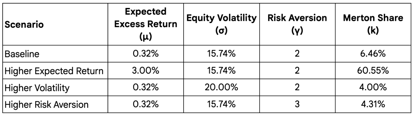
The “optimal” allocation to stock is listed in the last column (the Merton Share). As you can see the appropriate allocation to stocks is currently quite low. A higher equity risk premium of 3.00%, which is more in line with historical norms, provides roughly 10 times the allocation to stocks. That makes sense because the equity risk premium today is roughly 1/10th of 3.00% and we know that the allocation to stocks is a linear relationship.

The risk aversion (γ) component tells you that with a 3.00% equity risk premium, you would have an allocation close to the classic 60/40 stock/bond portfolio.

This table makes the Merton Share formula much clearer by showing how changes in expected excess return, volatility, and your personal risk aversion directly impact how much you should allocate to stocks. It visually confirms those direct and inverse relationships, helping you see how your own risk tolerance and market conditions should shape your portfolio.

For many people (including myself) the Merton Share just isn’t feasible. Do you know anyone willing to take just a 6.46% stake in the S&P 500? Even if you increase your risk aversion component to 1, you end up with a paltry 13% in stocks. Not what I would call practical!

However, firms like Elm Wealth, co-founded by Victor Haghani (who also co-wrote The Missing Billionaires), have used basic concepts from the Merton Share to build dynamic investment plans for their clients. Their strategies are rules-based and practical, allowing clients to personalize their portfolio to their own comfort levels, including how dynamic you want the portfolio to be.

Elm even recently launched an ETF that uses their strategies (ELM), which has quickly gathered a ton of capital. I encourage you to read Elm’s whitepaper and see if their strategy resonates with you.

That said, Elm Wealth’s full-blown strategy is usually for big-money investors ($2 million minimum), and while you may have access to their ETF at your broker, most 401Ks and some IRAs may have only limited options available. Nevertheless, understanding the Merton Share gives us a solid framework for building an asset allocation that is more rational, while Elm’s rules-based strategies can be adapted for DIY investors.

Before we discuss how to apply these principles in a more practical fashion, as with the CAPE ratio, we need to discuss some of the limitations of the Merton Share.

---

Limitations of the Merton Share in the Real World

Like any tool, the Merton Share is not perfect, especially when you try to apply it to the messy, unpredictable real world of investing. Furthermore, the Merton Share doesn’t always match up with practical limits of modern investing, even with increased market efficiency, lower fees, and many of the other benefits that weren’t available in Merton’s time. Here are just a few of the limitations:

• Constant Volatility: The basic Merton model assumes that market ups and downs (volatility) are always the same. In reality, market volatility is constantly changing, and those shifts can really mess with optimal asset allocation. While more advanced versions of the model try to account for this, it adds a ton of mathematical complexity.
• Continuous Rebalancing: The theory behind Merton Share assumes you’re constantly, continuously rebalancing your portfolio. In the real world, that’s just not possible because of trading costs and other logistical headaches. While frequent rebalancing (like Elm Wealth’s weekly adjustments) can get close, it’s still an approximation.
• Other Simplifications: The model also makes other simplifying assumptions, like a constant risk-free rate, stock prices moving in a predictable way, and a specific type of “utility function” (CRRA). These assumptions don’t always hold true in the complex, ever-changing financial markets.
• Quantifying Your Risk Aversion: Figuring out your risk aversion number (gamma) is tricky. This value isn’t stable or easily measurable like your height or weight. It can actually change depending on how the market’s doing — often dropping during bull markets when everyone feels confident and skyrocketing during market panics. While general ranges (like 1–5) or averages (like 2.5) are suggested, pinpointing it is a subjective challenge.
• Forecasting Returns: Even though the CAPE ratio gives us a solid long-term forecast for stock returns, future returns are always uncertain. So, the model’s effectiveness really depends on how accurate forward-looking estimates for both expected returns and volatility turn out to be.
• Potential Head-Scratchers: And here’s a head-scratcher: sometimes, the Merton Share might tell you to reduceyour stock exposure exactly when the market is going wild. Historically, those super volatile, scary times are often followed by the best returns, because that’s when you can snag the best deals.

Like the CAPE ratio, the Merton Share is a powerful idea, but it’s not a one-size-fits-all solution. It’s a theoretical ideal under specific, perfect conditions. Using it in the real world means you have to be smart about its limitations and understand the messy dynamics of markets.

The criticisms against the Merton Share, especially about its assumptions of predictable returns, continuous rebalancing, and the potentially counter-intuitive advice to reduce risk during highly volatile periods highlight a core tension between perfect theory and market reality. While the model is mathematically elegant for maximizing expected utility under its specific assumptions, these assumptions often don’t match what actually happens in the market.

In the third part of this discussion, we’ll discuss how to apply the Merton Share in a more practical and realistic fashion that doesn’t require constant monitoring and rebalancing or jumping in and out of the market. I’ll also provide a tool to help you determine the best asset allocation for you. See you then!

---